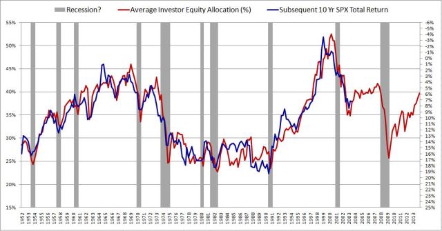
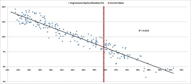
Consider the following chart, which shows the average investor portfolio allocation to equities from January 1952 to December 2013:
The metric in this chart takes no input from any variables traditionally associated with valuation: earnings, book values, profit margins, discount rates, etc. It consists only of a simple ratio between two numbers that can easily be calculated in FRED. Yet, as a predictor of future stock market returns, it dramatically outperforms all other stock market valuation metrics commonly cited.
In this piece, I’m going to do five things. First, I’m going to explain, in very simple terms, the accounting principles behind the metric. The explanation will include instructions (with ready-made links) for how to graph the metric in FRED. Second, I’m going to discuss the dynamics of asset supply, with a special focus on equities. Third, I’m going to challenge the conventional framework for understanding the relationship between valuation and stock market returns. Fourth, I’m going to introduce a new framework, one that relates stock market returns to equity asset supply. Fifth, I’m going to present a scatterplot of the predictive performance of the metric alongside other metrics, and discuss what the metric is currently forecasting for U.S. equity returns. I’m going to conclude by briefly touching on the question of whether or not the current U.S. stock market is “overvalued.”
Accounting Principles: Cash, Bonds, Stocks
To begin, let’s arbitrarily divide the universe of financial assets into three categories: (1) cash, (2) bonds, and (3) stocks. By “cash”, I mean bank deposits and circulating currency. By “bonds”, I mean any certificate of obligation to repay borrowed cash–commercial paper, bills, notes, bonds, etc. By “stocks” (or “equity”), I mean shares of ownership in a corporation (public or private). Note that these definitions are intentional simplifications.
Financial markets function on the following principle. For every unit of every financial asset in existence, some investor somewhere must willingly hold that unit in a portfolio at all times. By “investor”, I mean whoever owns wealth. There are intermediaries–hedge funds, mutual funds, pension funds, financial advisors, etc.–that help investors allocate wealth. But these entities are not the actual investors–their clients are.
The financial market is the place where investors decide–via trades–who will hold what units of what assets. Note that cash, as an asset, is special in that respect. It is the medium through which trades occur. Investors can only switch from one stock or bond to another stock or bond by going through cash. The going rate of exchange (bid or offered) between a unit of an asset and cash is the market price of the asset.
At the margin, if no investor can be found that wants to hold a given unit of a given asset at the prevailing market price, then the market price will fall until a willing holder is found. With respect to shares of a stock or bond, the application is straightforward. If no one wants to hold a given share at $100, then we try $95. Still no takers? Then we try $90, then $85, then $80, and so on. We continue until some investor emerges that finds the share sufficiently attractive to hold at the offered price. The concept applies analogously to cash–if no investor wants to hold cash, then the price that is bid on everything else will rise until everything else becomes so expensive and unattractive that some investor somewhere capitulates and agrees to hold cash instead. Measured in terms of other assets, the price of cash falls.
The “supply” of an asset is the total market value of it in existence–the total number of outstanding units times the market price of each unit. Put differently, supply is the amount of the asset available to be held in investor portfolios–the amount available for investors to allocate their wealth into. In aggregate, investors have to want to hold the total supply of each asset in existence in their portfolios. If there is too much supply of a given asset relative to the amount that investors want to hold in their portfolios, then the the market price of the asset will fall, and therefore the supply will fall. If there is too little supply of a given asset relative to the amount that investors want to hold in their portfolios, then the market price will rise, and therefore the supply will rise. Obviously, since the market price of cash is always unity, $1 for $1, its supply can only change in relative terms, relative to the supply of other assets.
The Aggregate Investor Allocation to Equities
Now, suppose that we open up every investor’s portfolio and calculate, for each investor, his percent allocation to stocks, bonds, and cash. My portfolio might be allocated 85% to stocks, 15% to bonds, 0% to cash. Yours might be allocated 50% to stocks, 20% to bonds, 30% to cash. And so on.
The question we want to answer is this: what would the average of all of these investors’ portfolio allocations look like, weighted by size? More specifically, what would the average investor allocation to stocks be? And how would that average compare to the averages of the past? It turns out that this question predicts the market’s future long-term returns better than any other classic valuation metrics to date developed–price to earnings (P/E), price to book (P/B), price to sales (P/S), CAPE, q-ratio, Market Cap to GDP, Fed Model, etc.
To answer the question, we need to know two things: (1) the total amount of stocks that investors in aggregate are holding, and (2) the total amount of cash and bonds that investors in aggregate are holding. Mathematically, the total amount of stocks that investors are holding divided by the total amount of everything (stocks plus bonds and cash) that they are holding just is the average investor allocation to stocks.
Now, to calculate the total quantity of cash and bonds in investor portfolios, we might think that we can just sum the total quantity of cash and bonds in existence outright–the total amount floating around the economy. After all, these securities have to be held by investors. But this approach won’t work. The reason is that a large portion of the bonds in existence are actually held by banks, not by investors. This fact extends to the central bank (the Federal Reserve), which presently owns an unusually large quantity of bonds.
Fortunately, there’s a convenient way to get around the problem. Recall that when the Federal Reserve buys bonds (treasury, MBS, etc.), it doesn’t add any net financial assets to investor portfolios. Rather, it takes bonds out of investor portfolios, and puts newly created cash into investor portfolios. It changes the cash-bond mix of the assets that investors hold–but not the total amount.
It turns out that private banks do essentially the same thing when they buy assets. They take the assets out of the hands of investors, and put their own liabilities–in the form of their own bonds or deposits (cash)–into investor hands. (They can also fund purchases with equity sales, but the equity component of a banks balance sheet is small enough to ignore.)
The entities that create net new financial assets (that investors can hold) are not banks, which are just intermediaries, but rather real economic borrowers. The universe of real economic borrowers consists of five categories: Households, Non-Financial Corporations, State and Local Governments, the Federal Government, and the Rest of the World. When these entities borrow directly from investors, the investors get new bonds to hold. When the entities borrow from banks, the investors get new cash to hold. That’s because when a bank makes a loan, the money supply expands. The loan creates a new deposit that didn’t previously exist–some investor must now hold that deposit in his portfolio of assets.
It follows, then, that if we want to get an estimate of the total amount of bonds and cash that investors are holding at any given time, all we have to do is sum the total outstanding liabilities of each of the five categories of real economic borrowers. Those liabilities either translate into cash that an investor somewhere is holding (if the entity took a loan from a bank, which expands the money supply), or they translate into a bond that an investor somewhere is holding (if the entity borrowed directly from the investor). Note that the average bond trades close to par (with some above, and some below), so, in aggregate, the value of the liabilities approximates the total market value of the bonds.
Banks don’t generally hold stocks. So to estimate the total amount of stocks in investor portfolios, what we need to know is the total market value of all stocks in existence. We end up with the following equation:
Investor Allocation to Stocks (Average) = Market Value of All Stocks / (Market Value of All Stocks + Total Liabilities of All Real Economic Borrowers)
We can get all of the information in this equation from the Flow of Funds report. The information is also conveniently available in FRED Graph. A link to the calculated metric is provided here, and to a separately downloadable version of each series, here.
Now, the Rest of the World creates an interesting complication. Parts of our portfolios are composed of stocks, bonds and cash denominated in foreign currencies (which do not show up in these series and are not being counted, though they should be). But in the same way, some parts of the portfolios of individuals in other countries are composed of stocks, bonds and cash denominated in our currency (which do show up in these series–and are being wrongly counted, given that our goal is to know our own allocations as domestic investors). As an estimation, it works to assume that the two cancel each other out.
The Unique Dynamics of Equity Asset Supply
The supply of cash and bonds that investors in an economy must hold perpetually increases with the economy’s growth. The cash and bonds in investor portfolios are literally “made from” the liabilities that real economic borrowers take on to fund investment–the fuel of growth.
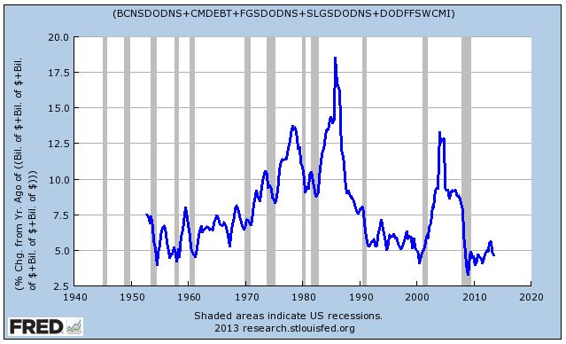
The following chart shows the annual growth of the total liabilities of all real economic borrowers–which, again, is the total supply of cash and bonds in investor portfolios–from 1952 to present. The growth rate has ranged anywhere from around 5% per year to around 15% per year. Right now, it’s at the low end of the spectrum.
Trivially, if the aggregate investor is going to maintain a constant portfolio allocation to equities, the supply of equities must grow commensurately with the supply of cash and bonds. Recall that investors, in aggregate, have to hold all of these assets at all times. It follows mathematically that the ratios of the total supplies outstanding must equal the ratios inside the “average” investor’s portfolio.
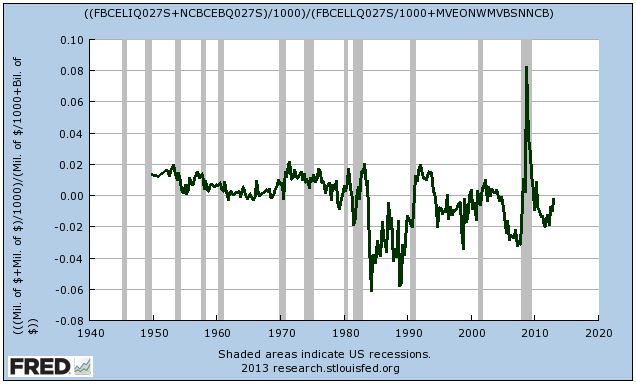
The supply of equities can increase in one of two ways: through the issuance of new shares, or through price increases, i.e., increases in the level of the stock market. The chart below shows the corporate sector’s net issuance of new equity, as a percentage of total market value, back to 1950.
As we see in the chart, the corporate sector is inherently averse to the issuance of new equity. Each year, it adds very little additional supply, on net. In various periods since the early 1980s, it’s actually been a net destroyer of equity supply–taking supply off the market through acquisitions and buybacks.
As we explained in our earlier piece on earningless bull markets, because the corporate sector does not issue sufficient amounts of new equity each year to keep up with the continually increasing supply of cash and bonds, stock prices have to rise over the long-term. If they don’t, stocks will become a smaller and smaller percentage of the aggregate investor portfolio. Unless investors, on average, want stocks to be a smaller component of their portfolios–because, for example, they increasingly prefer to hold other assets–this outcome will not be allowed. Stock prices will get pushed up on the growing relative scarcity until the aggregate equity allocation preference is satisfied.
Valuation: Challenging the Conventional Understanding
The total return of an equity security depends on two factors: (1) the change in price from purchase to sale, and (2) the dividends paid in the interim. Dividends matter, but price is king. It drives total return.
Many investors don’t like the fact that price drives total return. If price drives total return, it follows that total return is a function of the shifting sentiment, preferences and expectations of other people–those who make up the market and “vote” on what the price will be. Investors don’t want their returns to be subject to the arbitrary “vote” of other people, and so they pretend that as stock market speculators they are actually genuine businessmen who “buy” and “own” companies to hold forever. They tell themselves that their returns will somehow emerge directly from the cash flows of the underlying businesses, regardless of what the market decides to do with price.
This point of view ignores the fact that it takes decades to recoup an equity investment via dividends, the only cash flows that are ever are actually paid out to buy-and-hold investors. To claim a return on a stock in any other context, an investor needs someone to sell it to. The price that other people are wiling to pay is therefore important–supremelyimportant. Rather than resist this fact puristically, our responsibility as investors is to accept it and work within it, by understanding the behavioral propensities of our fellow market participants, and getting in front of emerging trends in how they choose to allocate their wealth.
Once we agree that price is king, the next question is: how is price determined in a market? Value mavens tend to think that price is determined through the “rational” application of normative valuation principles, such as “The stock market’s P/E ratio should be 15, plus or minus a few points. If interest rates are low, add a few points. If they are high, take a few points off.” On this view, when the actual P/E ratio is above the appropriate value, disciplined investors sell. When it’s below that value, they buy. Through their buying and selling, the price moves to where it “should” be, to “fair value”, given the earnings. Every so often, emotions disrupt the process, but as with everything, they eventually pass, and the process takes hold again. Value mavens look for these disruptions as an opportunity to capture excess return.
There’s certainly some truth to this view, but it doesn’t give the whole story. Ultimately, the price of equity is determined in the same way that the price of everything is determined–via the forces of supply and demand. For any given stock (or for the space of stocks in aggregate), price is always and everywhere produced by the coming together of those that don’t own the stock and want to allocate their wealth into it, and those that do own the stock and want to allocate their wealth out of it. If there is a different supply sought by the first group than offered by the second, the price will shift until the imbalance equalizes.
Now, there’s absolutely nothing that says that this process has to equilibriate at any specific valuation. History confirms that it can equilibriate at a wide range of different valuations. For perspective, the average value of the P/E ratio for the U.S. stock market going back to 1871 is 15.50. But the standard deviation of that average is a whopping 8.4,more than 50% of the mean. One standard deviation in each direction is worth 243% in total return, or 13% per year over 10 years.
The same is true of the popular Shiller CAPE. Its long-term average is 15.30–but with a standard deviation of 6.5, again almost 50% of the mean. Over the last 100 years, its value has stretched from as low as 5, to as high as 40–a difference of 700% in total return. Note that the periods in which it took on depressed values were hardly brief. It spent the entire decade of the 1940s at bargain basement levels, frequently falling into single digits–this in an environment where interest rates were pinned at zero.
Again, it’s all up to the allocators–they decide how much of their wealth they are going to allocate into stocks, how much exposure they are going to take on. Their preferences–or rather, their efforts to put those preferences in place, by buying and selling–set the price. Valuation is a byproduct of this process, not a rule that it has to follow. In the 1940s, investors decided, for whatever reason–memories of the Depression, a World War that the country might have lost, price controls, high inflation–that they didn’t want large stock market exposure. The fact that bond yields were meager did little to alter this preference. And so valuations stayed extremely depressed. When a vibrant, prosperous peacetime economy emerged in the 1950s, this preference obviously changed, and the biggest bull market in history ensued.
Buy-and-hold is painted as the informed, responsible, pro-American thing to do with a portfolio. But, in terms of financial stability, it can actually be a very destructive behavior. Consider the classic buy-and-hold allocation recommendation: 60% to stocks, 40% to bonds (or cash). What rule says that there has to be a sufficient supply of equity, at a “fair” or “reasonable” valuation, for everyone to be able to allocate their portfolios in this ratio? There is no rule.
If everyone were to jump on the buy-and-hold bandwagon, and decide to allocate 60/40, but equities were not already 60% of total financial assets, then they would necessarilybecome 60% of total financial assets. The excess bidding would not stop until they reached that level. It doesn’t matter that the associated price increase would cause the P/E ratio to rise to an obscenely high value. The supply-demand dynamic would force it to go there.
Now, in the real world, valuation concerns can and do push back on the equity allocation process. But, outside of extremes, they don’t tend to push back with very much force, at least not on their own. Let me now explain some of the reasons why.
We can divide asset allocators into two types: mechanical allocators, and active allocators. Mechanical allocators are individuals that adhere to a strict allocation formula, regardless of circumstance. Two examples would be buy-and-hold investors that are always 100% invested (or always 60/40 invested, periodically rebalancing, etc.), and 401K/retirement investors that invest automatically in accordance with a pre-defined program. These asset allocators follow their processes come rain or shine, therefore they cannot be relied upon to push back against valuation excesses. Though they are not the majority of the market, they are a significant part of it–their presence makes a difference.
Active allocators, in contrast, dynamically alter their allocations so as to maximize their returns. How do they try to maximize their returns? By allocating their wealth into the assets whose returns they consider to be the most attractive, adjusted for risk. It’s a competitive process–they choose among their options, based on their assessments of what those options are likely to produce.
Some might interpret this to mean that they look at the earnings yields on stocks, the yields to maturity on bonds, and the yield on cash, and then choose. Let’s suppose that asset allocation were this easy–just find the asset class with the highest yield, risk-adjusted, and allocate into it. We would still have to answer the question: what is the future yield (at the current price) of each asset class, adjusted for risk? To answer this question with respect to cash is hard–we have to estimate future short-term interest rates. With respect to bonds, even harder–we have to estimate credit risk. With respect to stocks, the hardest of all–we have to estimate forward earnings.
To estimate forward earnings for stocks, we have to answer difficult questions about the future: What will the trajectory of nominal growth be? How will profit margins evolve? Who can answer these questions with a significant degree of empirical confidence, enough to be a contrarian that consistently fights the market’s trends? Very few people, and therefore the answers to the questions end up reducing to biased reflections of prevailing mood, extrapolations of recent experience. When the mood is high, and when recent experience has been positive, investors embrace optimistic assessments of what the future holds–therefore, equities look cheap, attractive. The market gets the opposite of the valuation pushback that it needs. When the mood is low, and when recent experience has been negative, investors embrace more pessimistic assessments of what the future holds–therefore, equities look expensive, unattractive. Again, the market gets the opposite of the valuation pushback that it needs.
It turns out that even if fundamental questions about the future yields of cash, bonds, and equities were resolved, asset allocation still would not be as simple as choosing the security that offers the highest yield (risk-adjusted). The goal, again, is to maximize return. Return is not the same thing as yield.
Granted, if a security is held to maturity, or, in the case of equities, for an infinite period of time, the return will mathematically converge on the yield (provided, in the case of equities, that all earnings are eventually distributed as dividends). But who among us buys bonds to hold to maturity, or stocks to hold forever? Most investor time horizons are not on the order of decades, centuries or infinity, but on the order of days, months and years–a few days (the time horizon of a swing trader), a few months (the expiration date on a portfolio manager’s grace period with clients, at which point they will start leaving if things aren’t working), or a few years (long-term value investors playing with their own money).
To know the return of a security on a daily, monthly, or yearly time horizon, it’s not enough to know what the yields are. You need to know how the price is going to change. Given future cash flows (which we’ll assume you’ve accurately estimated), this requires knowing what the future valuation will be.
To illustrate, suppose that the P/E multiple on stocks is 20, the 10 year bond yield is 2%, and the rate on cash is 0%. Suppose further that the earnings of each of these securities are going to remain constant. Can you say which security will offer the highest return over the next few years? You might say stocks–the earnings yield is 5%, a healthy 3% more than bonds. The “premium” between the two is meaningfully higher than the historical average. But that doesn’t tell you what the return of stocks will be. If the investment mood sours ever so slightly over the next few years, and the market concludes that a P/E of 17 is more “appropriate” than a P/E of 20, the return will be negative–making stocks significantly less attractive than the other available assets, despite the higher earnings yield.
The only way that you can know what the future valuation of stocks will be–so as to estimate future returns–is to apply some conception of what’s fair, appropriate, reasonable, normal. But the range of what can be rationalized as fair, appropriate, reasonable, normal is extremely wide, too wide to be useful, and far too wide to provide reliable pushback against a supply-driven market advance. Any number that is chosen will likely be nothing more than a reflection of the prevailing allocation preference–the prevailing appetite to be in or out of the asset class, based on primordial “hunches” for where things are headed, themselves just manifestations of recency bias. Once again, the market will not get the valuation pushback that it needs.
Ultimately, valuation is a learned perception, learned through a process of social and environmental reinforcement. The part of it that is not learned is just a crude manifestation of the behavioral bias of anchoring–judging the attractiveness of a price (or a ratio) by comparing it to the price (or ratio) that one is “accustomed” to seeing. Ironically, it is anchoring, not “valuation discipline”, that keeps the market from doing crazy, bubbly things. People don’t like to pay higher prices tomorrow than they could have paid today, or sell for lower prices today than they could have sold for yesterday. That’s true regardless of what any valuation metric says.
To illustrate, suppose that you spend a significant amount of time in an environment where the average valuation is 25 times (or more). You acclimatize to that valuation, it becomes your anchor, what you are used to seeing. All of the “pundits” that you watch on TV tell you that it’s normal. All of your friends, your fellow investors, say that it’s normal. Most importantly, whenever you’ve bought at or below that valuation, it’s worked–the market has rewarded you with a positive outcome. And so you’re comfortable buying at that valuation.
Obviously, in such an environment, you will come to perceive 25 times earnings as a perfectly “appropriate” price for the market–a “fair” multiple. If given an opportunity to buy the market at a lower price–for example, 20 times–your reward circuitry will fire off, creating an appetite to lock in the “bargain”, jump on the “big gains” that it is offering.
But now switch the P/E in the example from 25 to 15. Suddenly, the same P/E of 20 will make you feel like you’re overreaching, exposing yourself to danger, buying too high. “Gee, what if the P/E falls back to 15, where it usually is, what I’m used to seeing–I’ll lose 25% in one move! I can’t afford that.”
Because valuation is a learned perception, driven by anchoring and by social and environmental feedback, it tends to follow the market. As valuations rise in a bull market, prior anchors wear off, and people get accustomed to higher valuations–over time, the valuations stop feeling “high”–making room for them to go even higher. Their perceived appropriateness gets reinforced–socially, in the market discussion, and environmentally, through the incredibly powerful feedback of actually making money. In a long, slogging bear market, the opposite occurs. Everything gets driven downwards.
To illustrate, consider the example of the most recent cycle. There was a time, before the crisis, when we talked about trailing P/Es of 18 or 19 times earnings as reasonable–maybe even a bargain, relative to the bubble that we had previously come out of. If we thought the trailing P/E was too high in the summer of 2007, we were told to ignore it–because the market was still very cheap on forward estimates (themselves just a reflection of the optimism).
Then, we had the Great Recession, a massive, negatively-reinforcing series of economic events–completely unrelated to stock market valuation, mind you–that shattered everyone’s equity world view. We suddenly found ourselves seriously debating whether 10 times trailing recessionary earnings was appropriate. We were supposedly in a “new normal”, which, we feared, implied structurally lower valuations.
The crisis eventually abated, and the economy entered a recovery. But people still had to work off their fear conditioning and their anchoring. As the market rose, the discussion shifted to whether 12 times was appropriate. Then, 14 times. Now, 17 times. The anchor, the goalpost, has continued to move with the market. Pretty soon, the discussion will come full circle again, and we will be asking ourselves whether 18 or 19 times is appropriate. And, if the cycle isn’t cut short by externalities, as it was the last time, we may one day find ourselves discussing the appropriateness of 25 times–which has been debated before in market history (a few years before the market proceeded to go to 40).
The drivers of this recurring pattern are obvious: not some innate “sense” of “fair value”, but anchoring and the social-environmental reinforcement of the market cycle itself. The perception of valuation is not capable of creating persistent, reliable resistance to the market cycle because it is an evolving function of the market cycle. At extremes, it can push back–but it can’t push back when it falls within the very wide range of what can be rationalized, which is where it usually falls, and where it is now.
Ultimately, we should be skeptical of claims that investors are innately hardwired to act in a certain way in response to any specific concept, argument, or data point–whether it be “valuation”, or anything else. Investors elicit behavioral responses to these types of informational inputs, but the responses are not innate. They are learned from the environment through a process of conditioning and reinforcement.
Investors attend to concepts, arguments, and data points, etc. as a means to an end–the end of predicting what the return will be, which, in practice, means predicting where the price is headed. If investors already have a hunch for where the price is headed–which they often do–they will choose to embrace whatever concepts, arguments, data points, etc. fit that hunch–or they’ll just ignore the “mumbo jumbo” altogether, and go with their “feel.” Similarly, if they are just using the constructs to save face in social debate–to avoid having to admit to themselves and to others that they are wrong–they will jump on whatever concepts, arguments, data points, etc. show that they are right (and ignore everything else).
When investors don’t have a hunch for where prices are headed, and are genuinely trying to use concepts, arguments, data points, etc. to assess what to do, the ensuing assessment ends up being something inherently insecure, subject to constant feedback and molding from the market–responsive to the result, and ditched when no longer working.
You might confidently think, for example, that “good jobs number” means “the recovery is picking up steam”, and that you should increase your equity risk–but if the market starts consistently telling you that this is wrong, by its actual result, you will be affected by the feedback. You may eventually find yourself pulled to function in accordance with the opposite rule, that “good is bad.” ”Maybe I shouldn’t rush to increase my exposure here. Maybe these good jobs numbers will lead the Fed to tighten–maybe that’s why the market is selling off. Oops.”
Admittedly, when enough people grab onto and act on concepts, arguments, data points, etc., they can become powerful forces that drive market outcomes, especially when they have a basis in reality that gives them credibility and forces people to believe them. The reflexivity of price confirmation increases their allure and persuasiveness, which causes more people to latch onto them, which fuels further price changes, therefore more price confirmation, and so on in a feedback loop that continues until reality pushes back.
However, it’s hard for valuation to pick up steam in this way, because unlike other themes that might move markets, it has no objective basis–it’s a personal opinion, easy to dismiss. It represents a resistance to what the market itself is doing–and is therefore already on the road to being disconfirmed simply by the fact that it is being raised. If valuations are too high, then why are we where we at them? Why aren’t we falling? Absent some kind of confirmation or feedback, the theme can’t go anywhere.
Outside of cyclical downturns in which profits themselves plunge, valuation never enters the discussion as a surprise, an “insult”, but rather is only introduced gently, gradually, as the market advances–usually by those who are not part of the advance. Market participants therefore have time to acclimatize to it as a theme. It can’t produce the kind of shock and surprise that would catch people offsides and provoke mounting, reflexively self-fulfilling reactions. That’s why it usually takes a recession–or some kind of noxious catalyst–to unwind a valuation excess. The excess alone can’t correct itself.
In the tech bull market, the overvaluation theme had a hard time pushing back even when index P/Es were in the 30s and 40s. People talked about overvaluation, they worried about it. But then they kept watching the price go up–so what do you do? You don’t tell the market that it’s wrong, you trust your environment, you go with the flow. In the end, it took a tight Fed, a recession with falling earnings, a slew of corporate bankruptcies and scandals, unfamiliar accounting changes that led to further earnings plunges, a terrorist attack, a war in the Middle East, and so on, to finally get the market moving reliably in the downward direction, so that the valuation excess could be corrected.
Asset Supply: A New Framework for Thinking About Equity Returns
Value mavens will tell you that the market’s P/E ratio (either simple trailing twelve months, or Shiller CAPE) is inversely correlated with future returns over the long-term. A high P/E ratio implies low future returns, a low P/E ratio implies high future returns.
But what makes this true? What is the force that brings about the inverse correlation? Recall that we said that equity total return is a function of price return and dividend return. We can aribtrarily separate price return into the part that comes from Earnings Growth, and the part that comes from the change in the P/E multiple. Leaving the mathintentionally imprecise, we end up with the following equations:
(1) Total Return = Price Return + Dividend Return
(2) Price Return = Price Return from P/E Multiple Change + Price Return from Earnings Growth (Realized if P/E Multiple Were to Stay Constant)
Combining (1) and (2):
(3) Total Return = Price Return from P/E Multiple Change + Price Return from Earnings Growth (Realized if P/E Multiple Were to Stay Constant) + Dividend Return
Now, suppose that the market has a P/E ratio of 100. Why does it have to produce a low or negative return? If corporate earnings are growing at the rate of nGDP, say 6%, and the P/E ratio stays at 100, then the return will be 6%–a perfectly healthy number.
Value mavens will respond that the P/E ratio cannot stay at 100. It mean-reverts over the long-term. Its mean-reversion is the basis for its inverse correlation with long-term future returns. If you buy at a price below the normal P/E range, you will get the dividend return, plus the return from earnings growth, plus the boost from multiple expansion. Thus your return will be higher than normal. Conversely, if you buy above the normal range, you will get the dividend return, plus the return from earnings growth–but those two gains will then be offset by losses from multiple contraction. Thus your total return will be lower than normal.
The problem with this construction, of course, is that it doesn’t model the real reasons that stock prices, in aggregate, change. Stock prices don’t change because market participants choose to assign stocks different P/E multiples. Rather, they change because the eagerness of the aggregate investment community to allocate wealth into stocks rises or falls. More investors try to “put money to work” than try to “take money off the table”, and vice-versa. In the presence of the imbalance, the price has no choice but to change.
As equity investors, we talk a lot about asset allocation. It’s essentially the most important aspect of portfolio management–how we’re allocated within the space of individual stocks and bonds, and across the space of assets in general. I’m 85% equity, 15% cash/bonds. You’re 50% equity, 50% cash/bonds. Joe over there is 100% equity, 0% cash/bonds, etc.
What’s funny is that we never think to ask: how is it possible for all of us to get to within a reasonable range of these preferred allocations at the same time? After all, we’re trading a limited supply of things amongst each other. The answer, of course, is that the supply, properly understood, automatically shifts to meet our allocation preferences via the changes in price that we cause when we try to put those preferences in place–that is, when we buy and sell at the margin. In bull markets, we frequently find ourselves searching for opportunities to put our allocation preferences in place–our equity exposures are rarely as high as we would like them to be.
I therefore propose a new way of framing equity total returns. Take the previous equation, and substitute “Aggregate Investor Allocation to Stocks” and “Increase in Supply of Cash and Bonds” for ”P/E Multiple Change” and “EPS Growth.” We then have,
(1) Total Return = Price Return + Dividend Return
(2) Price Return = Price Return from Change in Aggregate Investor Allocation to Stocks + Price Return from Increase in Cash-Bond Supply (Realized if Aggregate Investor Allocation to Stocks Were to Stay Constant) + Dividend Returns
Combining (1) and (2),
(3) Price Return = Price Return from Change in Aggregate Investor Allocation to Stocks + Price Return from Increase in Cash-Bond Supply (Realized if Aggregate Investor Allocation to Stocks Were to Stay Constant) + Dividend Return
In the previous way of thinking, the earnings grow normally as the economy grows. If the multiple stays the same, the price has to rise–this price rise produces a return. When the multiple increases alongside the process, the return is boosted. When it decreases, the return is attenuated. The multiple is said to be mean-reverting, and therefore when you buy at a low multiple, you tend to get higher returns (because of the boost of subsequent multiple expansion), and when you buy at a high multiple, you tend to get lower returns (because of the drag of subsequent multiple contraction).
In this new way of thinking, the supply of cash and bonds grows normally as the economy grows. If the preferred allocation to stocks stays the same, the price has to rise (that is the only way for the supply of stocks to keep up with the rising supply of cash and bonds–recall that the corporate sector is not issuing sufficient new shares of equity to help out). That price rise produces a return. When the preferred allocation to equities increases alongside this process, it boosts the return (price has to rise to keep the supply equal to the rising portfolio demand). When the preferred allocation to equities falls, it subtracts from the return (price has to fall to keep the supply equal to the falling portfolio demand).
Now, instead of saying that the P/E multiple is mean-reverting, we say that, for a given set of environmental contingencies–e.g., history, culture, demographics, etc.–theequity allocation preference is mean reverting. It rises in expansionary parts of the cycle, as people become more optimistic about the future and more eager to maximize what they see as attractive returns (“Kelly, we believe in this bull market, we’re fully invested, our clients are fully invested.”–something you hear frequently on CNBC these days), and it falls in contractionary parts of the cycle, as people become less optimistic about the future and more concerned about protecting themselves from losses (“Maria, we’re cautious here, we’ve raised cash, we want to see signs of stabilization before we deploy it.”–something that you heard frequently on CNBC in ’08 and early ’09).
If you buy in periods where the investor allocation to equities is low, you will get the dividend return plus the price return necessary to keep the portfolio equity allocation constant in the presence of a rising supply of cash and bonds, plus the price return that will occur when equity allocation preferences return to more normal levels. You will get in front of the equity supply squeeze of the next bull market, when risk appetite and the associated desire to be invested in equities recovers. Thus your return will be higher than normal. This is what happened to investors in the 1980s.
If you buy in periods where the investor allocation to equities is high, you will get the dividend return plus the price return necessary to keep the portfolio equity allocation constant in the presence of a rising supply of cash and bonds, but then you will have to subtract the negative price return that will occur when equity allocation preferences fall back to more normal levels. This is what happened to investors in the 2001-2003 bear market.
This way of thinking about stock market returns accounts for relevant supply-demand dynamics that pure valuation models leave out. That may be one of the reasons why it better correlates with actual historical outcomes than pure valuation models.
It can explain, for example, the earningless bull market of the 1980s. Unbeknownst to many, earnings were not rising in the 1980s bull market. They actually fell slightly over the period–which is unusual. But prices didn’t care–they skyrocketed. The P/E ratio ended up rising well above 20, despite interest rates near 10%–a valuation disparity never before seen in history. Valuation purists can’t explain this move–they have to postulate that the “common sense” rules of valuation were temporarily suspended in favor of investor craziness.
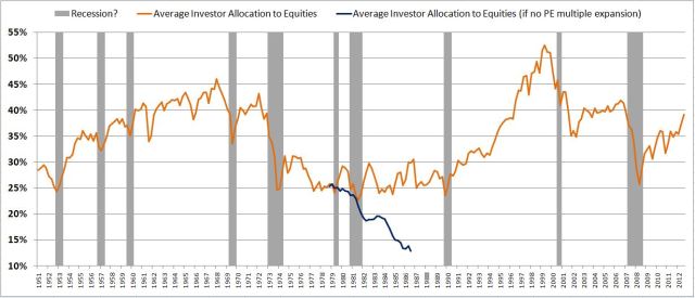
But if we look at what investor allocations were back then, we will see that investors were already dramatically underinvested in equities. If prices hadn’t risen, if investors had instead respected the rules of “valuation” and refrained from jacking up the P/E multiple, the extreme underallocation to equities would have had to have grown even more extreme. It would have had to have fallen from a record low of 25% to an absurd 13% (see blue line in the chart below, which shows how the allocation would have evolved if the P/E multiple had not risen). Obviously, investors were not about to cut their equity allocations in half in the middle of a healthy, vibrant, inflation-free economic expansion–a period when things were clearly on the up. And so the multiple exploded.
Now, recognize that this framework leaves plenty of room to acknowledge the relevance of classical valuation considerations. Disparities in valuation–between equities and their own history (the valuation levels investors are anchored to, accustomed to seeing, that they consider to be “normal”) and between equities and other asset classes (bonds and cash)–can certainly cause investors to want to change their allocations and exposures, especially when the disparities are significant and can’t be dismissed or rationalized away. If such a change unfolds, prices will rise or fall accordingly. But if such a change doesn’t unfold, then prices are not going to respond. Nor “should” they.
In a way, the metric already offers a rough estimation of classical valuation. If the average investor allocation to equities is abnormally low, then prices are probably abnormally low–the market’s probably cheap. Likewise, if the average investor allocation to equities is abnormally high, then prices are probably abnormally high–the market’s probably expensive. And so an investor that is value-sensitive can still use the metric as a way of assessing the market opportunity.
Comparing the Metrics on Performance
The following chart is a scatterplot of the new metric. The y-axis is 10 year SPX total return, the x-axis is the average investor equity allocation. The solid red line is the current value of the metric. Note the excellent fit.
Right now, at its current value, the metric suggests a future 10 year nominal total return for equities of around 6%. Historically, whenever the market was at the current level, the low end of the return was a tad less than 5%, and the high end was around 9%.
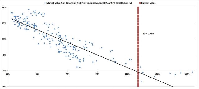
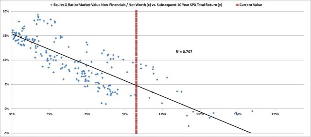
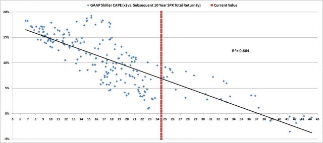
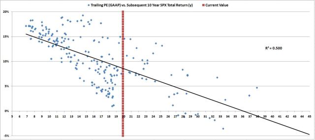
The following charts show scatterplots of the other metrics. It’s not even worth speculating on what returns they are suggesting right now, because the fits are atrocious, especially in the current valuation range. The Equity Q-ratio, for example, puts the market’s current future 10 year returns anywhere from as low as 2% to as high as 9%. The Shiller CAPE puts the returns anywhere from as low as 0% to as high as 10%–with an ironic bias to the upside. Market Cap to GDP puts returns anywhere from -3% to 2%(which is why it has become fashionable among bears).
In our earlier piece, we pointed out that the classic Shiller CAPE wrongly labeled the March 2003 market as significantly overvalued, and the March 2009 market as barely below fair value (an epic, inexcusable blunder). We pointed out that one advantage of the pro-forma CAPE, which tried to eliminate accounting inconsistencies, was that it correctly identified the market’s attractive valuation in these periods. It called March 2003 a decent value, and March 2009 a screaming buy.
It turns out that like the pro-forma CAPE, this metric also called 2003 and 2009 correctly. It signaled the March 2003 market as a reasonable buy, and the March 2009 market as a screaming buy, on par with levels seen at the secular low of the last bear market, 1982.
A Note on “Overvaluation”
There’s a raging debate right now between bulls and bears over whether the U.S. stock market is presently overvalued. The debate rages on because the term is poorly defined. What, precisely, does it mean to say that something is “overvalued”?
When we say that the stock market is “overvalued”, we might mean that it’s currently valued more expensively than it typically has been in the past. Over its history, the U.S. stock market has offered, on average, some expected total return–say 8% to 10%. But now it’s priced for 5% or 6% (using our metric). So it’s “overvalued.”
Fair enough, bulls shouldn’t disagree. There are tons of reasons why the present stock market is unlikely to produce the 8% to 10% returns that it has produced, on average, throughout history. On almost every relevant measure, it’s starting out from a higher-than-average level.
The more important question, however, is this: why should the stock market offer investors the average historical return right now? If, over the next 10 years, bonds are offering investors 2.8%, and cash is offering them less than 1%, why should stocks be priced to offer them 8% to 10%?
How would that even be sustainable? If equities were offering an 8% to 10% return, we would all choose to allocate the bulk of our portfolios into them, rather than languish in the ZIRPY nothingness of bonds and cash. There obviously isn’t enough equity supply for all of us to allocate in that way, and so the price would get pushed up, and the expected return pulled down–very quickly.
Now, it’s a mistake, obviously, to make an assessment of valuation based strictly on a comparison between the yields of stocks and bonds, as the Fed Model suggests we do. The yield of an equity security, again, is not the same as its return. You can buy the market at 33 times earnings–a 3% earnings yield–but your return over the next 10 years isn’t going to be 3%. It will probably be 0% (or less), as the market contracts from the obscene valuation at which you bought it. If you were to try to justify the stock market’s price by comparing its 3% yield to the 10 year bond yield at 1%, touting the healthy risk premium (2%–greater than the historical average), you would obviously be making a huge mistake. The real risk premium on your stock investment would be negative–you would end up with a loss.
But if you properly estimate long-term equity returns using other methods–for example, the method I’ve proposed, which puts the future return for the stock market at 5% to 6%–then it makes perfect sense to assess the “appropriateness” of the current valuation through a process of comparison with the investment alternatives. In the current case, the alternatives of cash and bonds are offering much less than 5% to 6%–so there’s a decent risk premium in place for equities. The market is not “overvalued”–it doesn’t “belong” at a lower valuation. To the contrary, it’s priced where it should be, given the alternatives. Investors have done their jobs properly, leaving no easy arbitrages to exploit.
Now, if bears want to argue that it’s unwise to lock in 5% to 6% equity returns right now (or even 3% or 4%), because the market cycle will eventually produce selloffs in which greater returns are made available, my response would be: who said anything about locking anything in? Let’s time the market–as bears seem to want to do. I’m all for that approach.
But timing the market doesn’t mean boycotting it until it hands you, on a silver platter, the high returns that you’re demanding. After all, there’s an excellent chance that it won’t hand them to you–there’s no reason it has to. General societal progress–particularly in the area of economic policymaking–reduce the odds that it will. Rather, timing the market means monitoring for the types of processes that tend to cause markets to sell off–capturing equity returns except when there are signs of those processes emerging. “Valuation”–at least in the range that we’re currently at–is not one of the processes that cause markets to sell off (or, for that matter, that stop markets from selling off). So stop worrying about it.
Big selloffs usually occur in association with recessions. That’s where market timers make their money–by anticipating turns in the business cycle. A hint to bears: if you’re calling for a recession right now, in this monetary environment, you’re doing it wrong.
